About This Site

Posted Oct 28, 2018

Abstract

The season of American football is back, and with it the Fantasy, the already traditional online game which you bring your friends or coworkers to play together in a virtual league, where each member rosters NFL’s players on virtual teams and hoping that they will score well in their real life games. The real life player’s score goes to your virtual team score.

ffanalytics package

The PhD in clinical psychology and assistant professor Isaac Petersen author of the site Fantasy Football Analytics, who does projections and analysis of Fantasy results, did a great job with the ffanalytics package made available in GitHub.

This package does data scrapping in various sites that make predictions of player’s performances such as ESPN, CBS, Yahoo and the NFL website itself, after, applies the fantasy scoring rules (which can even be cutomized for your League) and calculates the score possible for each of the projections.

Finally, the package analyzes the points obtained by making performance projections of the results, aggregating in one vision the predictions of several sites. Isaac publishes weekly the ranking of projections by position for the games of the round, using some standards scoring rules.

With all the hard work of doing data scrapping and apply the rules of fantasy to calculate the score already made by the package, we can use these informations to project the results of teams scaled in fantasy leagues and to forecast game results, remaining only to obtain the teams and their rosters from Fantasy itself.

Fantasy API - Getting the Team’s Matchups and Rosters

In order to obtain the rounds of a fantasy league, we can use the Web API available by the Fantasy website. Although it has some depreciated methods they still work and serve the purpose of getting the information we want. In particular we need access the methods that tells us which games /league/matchups is schedule for a week. This API receives as input parameters the authentication token, theid of the league and the week of interest, returning the games scheduled for that week. We also will use the API /league/team/matchup that, in addition to the above parameters, also gets the team id to return the team roster.

We can invoke the API using the httr package and process the response json usingjsonlite.

# Storing the Access Token and League ID locally
# I use a yalm file to avoid hard-code them 
# or eventually version them in the GitHub :)
library(yaml)

config <- yaml.load_file("../../../config/config.yml")
leagueId <- config$leagueId
authToken <- config$authToken

# invoking the API
library(httr)
library(glue) # to easily replace vars in the url

# league/matchups url
url <- "http://api.fantasy.nfl.com/v1/league/matchups?leagueId={leagueId}&week={week}&format=json&authToken={authToken}"
week <- 5

# call the api
resp <- httr::GET(glue(url))

# Is it ok?
resp$status_code

## [1] 200

Once the call response is obtained, we treat the return * json * to organize the data and obtain the team rosters.

library(jsonlite)
library(tidyverse)
library(kableExtra)

# to convert the json in a "tabular-tibble form"
resp %>% 
  httr::content(as="text") %>%
  fromJSON(simplifyDataFrame = T) %$%  
  leagues %$%
  matchups %>%
  .[[1]] %>% 
  jsonlite::flatten() %>% 
  as.tibble() -> matchups

 matchups %>% 
   select(awayTeam.id, awayTeam.name, homeTeam.name, homeTeam.id) %>% 
   kable() %>%
   kable_styling(bootstrap_options = "striped", full_width = F)

awayTeam.id	awayTeam.name	homeTeam.name	homeTeam.id
1	Change Robots	Rio Claro Pfeiferians	6
7	NJ’s Bugre	Sorocaba Steelers	5
11	Campinas Giants	Amparo Bikers	4
2	Sorocaba Wild Mules	Indaiatuba Riders	3

We make new calls to the API to get the roster of each team in that week.

# for each teamIds in the matchup
c(matchups$awayTeam.id) %>%
  map(
    function(.teamId, .week, .leagueId, .authToken, .url) {
      # make the API call
      httr::GET(glue(.url)) %>%
        httr::content(as = "text") %>%
        fromJSON(simplifyDataFrame = T) %>% # transform response body in json
        return()
    },
    .week      = week,
    .leagueId  = leagueId,
    .authToken = authToken,
    .url       = "http://api.fantasy.nfl.com/v1/league/team/matchup?leagueId={.leagueId}&teamId={.teamId}&week={.week}&authToken={.authToken}&format=json"
  )  -> rosters.json

# this is a list with the team rosters used in this week
rosters.json[[1]]$leagues$matchup$homeTeam$name

## [1] "Rio Claro Pfeiferians"

rosters.json[[1]]$leagues$matchup$homeTeam$players[[1]] %>%
  select(id, name, position, teamAbbr) %>% 
  as.tibble() %>% 
   kable() %>%
   kable_styling(bootstrap_options = "striped", full_width = F)

id	name	position	teamAbbr
2558125	Patrick Mahomes	QB	KC
2507164	Adrian Peterson	RB	WAS
2543773	James White	RB	NE
2508061	Antonio Brown	WR	PIT
2556370	Michael Thomas	WR	NO
2558266	George Kittle	TE	SF
2555430	Alex Collins	RB	BAL
1581	DeSean Jackson	WR	TB
2540158	Zach Ertz	TE	PHI
2540160	Jordan Reed	TE	WAS
2558063	Deshaun Watson	QB	HOU
2558865	Chris Carson	RB	SEA
2559169	Austin Ekeler	RB	LAC
2507232	Mason Crosby	K	GB
100011	Green Bay Packers	DEF	GB

With the team’s rosters (json format) we process the data to facilitate the handling.

# auxiliar transformation to extract team roster
extractTeam <- . %>% 
  .$players %>% 
  .[[1]] %>% 
  select( src_id=id, name, position, rosterSlot, fantasyPts ) %>%
  jsonlite::flatten() %>% 
  as.tibble() %>% 
  select(-fantasyPts.week.season, -fantasyPts.week.week ) %>% 
  rename(points = fantasyPts.week.pts) %>% 
  mutate(
    src_id = as.integer(src_id), 
    points = as.numeric(points)
  )

# extract each roster
rosters.json %>% 
  map(function(.json){
    matchup <- .json$leagues$matchup
    tibble(
      home.teamId = as.integer(matchup$homeTeam$id),
      home.name   = matchup$homeTeam$name,
      home.logo   = matchup$homeTeam$logoUrl,
      home.pts    = as.numeric(matchup$homeTeam$pts),
      home.roster = list(extractTeam(matchup$homeTeam)),
      away.teamId = as.integer(matchup$awayTeam$id),
      away.name   = matchup$awayTeam$name,
      away.logo   = matchup$awayTeam$logoUrl,
      away.pts    = as.numeric(matchup$awayTeam$pts),
      away.roster = list(extractTeam(matchup$awayTeam))
    ) %>% 
      return()
  }) %>% bind_rows() -> matchups.rosters

# check the matchups QBs for each team 
matchups.rosters %>% 
  mutate( away.qb = map(away.roster, function(roster) roster %>% filter(rosterSlot=="QB")),
          home.qb = map(home.roster, function(roster) roster %>% filter(rosterSlot=="QB")) ) %>%
  unnest(away.qb, home.qb, .sep=".") %>% 
  select(away.team = away.name, away.qb.name, home.qb.name, home.team=home.name ) %>% 
   kable() %>%
   kable_styling(bootstrap_options = "striped", full_width = F)

away.team	away.qb.name	home.qb.name	home.team
Change Robots	Aaron Rodgers	Patrick Mahomes	Rio Claro Pfeiferians
NJ’s Bugre	Russell Wilson	Ben Roethlisberger	Sorocaba Steelers
Campinas Giants	Tom Brady	Drew Brees	Amparo Bikers
Sorocaba Wild Mules	Matt Ryan	Cam Newton	Indaiatuba Riders

Now we have a tibble with the games between the teams and, nested in each registry, the respective rosters. Now you will need to use ffanalytis package to get the prediction performance and score of each player.

Forecast players perform

Firstly, we will use the ffanalytics package to do the data scraping of the forecasts for each player in the league made by the main sites that follow and make this type of prediction.

library(ffanalytics)
scrap <- scrape_data(pos = c("QB", "RB", "WR", "TE", "K", "DST"),
                     season = 2018,
                     week = week)

The scrape_data function returns a list by position, with the performance projections of the players in that position. This is because the predictions for each position have different attributes, for example, Kickers are evaluated by the number of field goals and distances of the kicks, and Quaterbacks by the numbers and distances of the passes.

# Quaterback Projection Attributes
scrap$QB %>%  
  filter(player=="Drew Brees") %>% 
  select(4:10) %>% 
   kable() %>%
   kable_styling(bootstrap_options = "striped", full_width = F)

player	team	pass_att	pass_comp	pass_yds	pass_tds	pass_int
Drew Brees	NO	37.60	26.10	287.00	2.00	0.70
Drew Brees	NO	37.30	26.20	272.70	1.70	0.60
Drew Brees	NO	38.20	26.50	305.00	1.90	0.60
Drew Brees	NO	44.00	29.00	305.00	3.00	1.00
Drew Brees	NO	38.20	26.60	305.00	2.00	0.60
Drew Brees	NO	39.51	25.99	309.47	2.51	0.63
Drew Brees	NO	NA	NA	283.36	1.94	0.73

# Kickers Projection Attributes
scrap$K %>%  
  filter(player=="Justin Tucker") %>% 
  select(4:10) %>% 
   kable() %>%
   kable_styling(bootstrap_options = "striped", full_width = F)

player	team	fg	fg_att	fglg	xp	xpatt
Justin Tucker	BAL	1.80	1.90	0	2.60	2.6
Justin Tucker	Bal	1.90	2.00	NA	2.20	NA
Justin Tucker	BAL	2.00	2.30	NA	2.30	NA
Justin Tucker	BAL	2.00	NA	NA	3.00	NA
Justin Tucker	BAL	1.86	2.25	NA	2.29	NA
Justin Tucker	Bal	NA	NA	NA	2.50	NA
Justin Tucker	BAL	NA	NA	NA	1.94	NA

Secondly, with projections in hand, we use ffanalytics package again to calculate how many points each player will make according with each prediction scraped from the sites. However, the package does not export the function that does the this individual calculation, but it is a necessary step to calculate the projections table that the site uses in its graphics.

But the package project is in the GitHub, so, it is possible to download the code, load the scripts directly and access the function that calculates the points per player and projection site. The function is called source_points(), and is present in the script calc_projections.R. You can load the script (and its dependencies) to invoke it directly.

# function to access 'source_points' directly
playerPointsProjections <- function(.scrap, .score_rules){
  source("../ffanalytics/R/calc_projections.R")
  source("../ffanalytics/R/stats_aggregation.R")
  source("../ffanalytics/R/source_classes.R")
  source("../ffanalytics/R/custom_scoring.R")
  source("../ffanalytics/R/scoring_rules.R")
  source("../ffanalytics/R/make_scoring.R")
  source("../ffanalytics/R/recode_vars.R")
  source("../ffanalytics/R/impute_funcs.R")
  source_points(.scrap, .score_rules)
}

# customized scoring rules
source("./score_settings.R") 
players.points <- playerPointsProjections(scrap, dudes.score.settings)

pos	data_src	id	points
K	CBS	8359	10
K	CBS	12956	9
K	CBS	11936	9
K	CBS	6789	9
K	CBS	8930	9
K	CBS	11384	9

Merging Rosters and Predictions

We now have the teams rosters and the scoring projections of the sites for each player, so we need to join the datasets. But to do that it is necessary to match the players’ ids. If you notice the data displayed, each player’s ID is different on each of the sites, ffanalytics package names this id as src_id, but unifies the results to a unified, identificator named id.

The teams’ rosters were obtained from the fantasy site, it follows the src_id identification of the NFL, to make the merge between the two dataset it will be necessary to map the src_id of the NFL to id of ffanalytics package. We can extract this ‘ids’ mapping from NFL prediction scraped data:

# look the presence of both ids in the projection table
scrap$WR %>% 
  filter( data_src=="NFL" ) %>% 
  select(1:4) %>% 
  head() %>% 
   kable() %>%
   kable_styling(bootstrap_options = "striped", full_width = F)

data_src	id	src_id	player
NFL	11675	2543495	Davante Adams
NFL	12181	2552600	Nelson Agholor
NFL	10651	2530660	Kamar Aiken
NFL	11222	2540154	Keenan Allen
NFL	9308	2649	Danny Amendola
NFL	12930	2556462	Robby Anderson

# extracting id and src_id from all positions
scrap %>%
  map(function(dft){
    dft %>% 
      filter(data_src=="NFL") %>% 
      select(id, src_id, player, team, pos) %>% 
      return()
  }) %>% 
  bind_rows() %>%
  distinct() -> players.ids

# ID mapping
head(players.ids) %>% 
   kable() %>%
   kable_styling(bootstrap_options = "striped", full_width = F)

id	src_id	player	team	pos
13589	2560955	Josh Allen	BUF	QB
13125	2557922	C.J. Beathard	SF	QB
11642	2543477	Blake Bortles	JAX	QB
9817	497095	Sam Bradford	ARI	QB
5848	2504211	Tom Brady	NE	QB
4925	2504775	Drew Brees	NO	QB

Finally we can make the predictions merging of players to the team’s rankings.

# nest by "id" and merge with "src_id"
players.points %>% 
  select(-pos) %>% 
  group_by(id) %>% 
  nest(.key="points.range") %>%
  # merge ID with SRC_ID
  inner_join(players.ids, by = c("id")) %>%
  select(id, src_id, player, pos, team, points.range) %>% 
  # keep only "ids" at top level
  select(id, src_id, points.range) -> players.ids.points

# auxiliary function to merge roster with player points
mergePoints <- function(.roster, .points){
  .roster %>% 
    left_join(.points, by="src_id") %>% 
    return()
}

# merge points in rosters
matchups.rosters %>% 
  mutate(
    home.roster = map(home.roster, mergePoints, .points=players.ids.points),
    away.roster = map(away.roster, mergePoints, .points=players.ids.points)
  ) -> matchups.points

Note that we are using a structure of nested data.frames, i.e., we have a matchups data.frame where each line is a match. In each match there are two rosters columns (“home” and “visitor”), these columns hold another data.frame, containing the roster itself. In this data.frame, each line is a player, and for each player there is a column called points.range which also contains another data.frame, with the prediction of each site’s player scores.

# "father" dataframe and the first nested column
matchups.points %>% 
  select( home.name, home.roster )

## # A tibble: 4 x 2
##   home.name             home.roster      
##   <chr>                 <list>           
## 1 Rio Claro Pfeiferians <tibble [15 x 7]>
## 2 Sorocaba Steelers     <tibble [15 x 7]>
## 3 Amparo Bikers         <tibble [15 x 7]>
## 4 Indaiatuba Riders     <tibble [15 x 7]>

# seeing the first nested data.frame
matchups.points[1,]$home.roster[[1]]

## # A tibble: 15 x 7
##     src_id name            position rosterSlot points    id points.range   
##      <int> <chr>           <chr>    <chr>       <dbl> <int> <list>         
##  1 2558125 Patrick Mahomes QB       QB           15.8 13116 <tibble [9 x 2~
##  2 2507164 Adrian Peterson RB       RB            4.2  8658 <tibble [9 x 2~
##  3 2543773 James White     RB       RB           13.7 11747 <tibble [9 x 2~
##  4 2508061 Antonio Brown   WR       WR           22.1  9988 <tibble [9 x 2~
##  5 2556370 Michael Thomas  WR       WR            7.4 12652 <tibble [9 x 2~
##  6 2558266 George Kittle   TE       TE            8.3 13299 <tibble [9 x 2~
##  7 2555430 Alex Collins    RB       W/R           6.6 12628 <tibble [8 x 2~
##  8    1581 DeSean Jackson  WR       BN            0    9075 <tibble [4 x 2~
##  9 2540158 Zach Ertz       TE       BN           17   11247 <tibble [10 x ~
## 10 2540160 Jordan Reed     TE       BN            2.1 11248 <tibble [9 x 2~
## 11 2558063 Deshaun Watson  QB       BN           21   13113 <tibble [9 x 2~
## 12 2558865 Chris Carson    RB       BN           12.7 13364 <tibble [8 x 2~
## 13 2559169 Austin Ekeler   RB       BN           11.9 13404 <tibble [6 x 2~
## 14 2507232 Mason Crosby    K        K             3    8742 <tibble [10 x ~
## 15  100011 Green Bay Pack~ DEF      DEF           2     523 <tibble [8 x 2~

# look the second level dataframe
matchups.points[1,]$home.roster[[1]][1,]$points.range[[1]]

## # A tibble: 9 x 2
##   data_src      points
##   <chr>          <dbl>
## 1 CBS             16  
## 2 ESPN            18.7
## 3 FantasyPros     22.3
## 4 FantasySharks   19.5
## 5 FFToday         20.5
## 6 FleaFlicker     24.7
## 7 NFL             19.1
## 8 NumberFire      24.6
## 9 Yahoo           18.8

Nested data.frames is a convenient model because it allows you to keep the data together and manipulate them easily.

Monte Carlo Simulation

To simulate the result of round matches, we need to simulate the score obtained by each teams and for this we will simulate the score of the team members using Monte Carlo simulation.

To simulate the players’ scores we will consider that each of the players can make one of the scores projected by the forecast sites. For simplicity, in this post, we can assume that the odds are equal for any of the projected scores.

In this case the simulation of a match using Monte Carlo then consists in:

For each player of the team, draws one of the possible projected numbers
We sum the players’ points drawed: this will be the team score
Compare the score of the home team with the away team to determine who won
A win is computed for the team with the highest score

This procedure is repeated N times, simulating several matchs, to determine the chances of winning a team, we sum the total number of times in which the team was a winner and divide by the total number of simulations. Thus we will have the chances of each team winning the match, once the simulations reflect the numerous combinations of scores between players and their teams.

Note that we assume that each player has equal chance of having any of the projected scores as a simulation score, more sophisticated models could consider different ranges with different probabilities between projections, including assessing the performance history of the site, but I’ll leave this considerations to another future post.

### Auxiliary functions

# function to generate .n possible pontuations from .points.range
# it's used to generate the .n simulations to each player
simPlayer <- function(.points.range, .n){

  # just check if the points.range isn't empty
  if(is.null(.points.range)) return( vector(mode = "numeric",.n) )
  if(nrow(.points.range)==0) return( vector(mode = "numeric",.n) )

  # generate a .n vector samples from points.range
  .points.range$points %>% 
    sample(size = .n, replace = T) %>%
    return()

}

# function to add the player pontuation to the team roster dataframe
simTeam <- function(.roster, .n){
  .roster %>% 
    mutate( sim.player = map(points.range, simPlayer, .n=.n) )  %>% 
    return()
}

# this function is in charge to sum the pontuations from 
# each player to generate the .n-size vector with team pontuation
simTeamPoints <- function(.roster){
  .roster %>% 
    filter(rosterSlot!="BN") %>%  # exclude player in bench
    pull(sim.player) %>%          # get the player pontuation simulation
    bind_cols() %>%               # binds the pontuation toghether 
    as.matrix() %>%               # now we have an matrix with # players x # .n simulations
    rowSums(na.rm = T) %>%        # sum each row (simuilation) to get a .n-vector 
    return()                      # each position in this vector is a possible team pontuation
}

### Simulation Code

# number of simulations
n <- 2000

# in the matchups dataframe
matchups.points %>% 
  mutate(
    # just team nicknames to shorter legends :)
    away.nickname = gsub("([a-zA-Z\']+ )?", "", away.name),
    home.nickname = gsub("([a-zA-Z\']+ )?", "", home.name)
  ) %>% 
  mutate(
    home.roster  = map(home.roster, simTeam, .n=n), # add players simulation points
    away.roster  = map(away.roster, simTeam, .n=n), # to each roster
    home.sim.pts = map(home.roster, simTeamPoints), # computes the team simulation
    away.sim.pts = map(away.roster, simTeamPoints)  # points
  ) %>% 
  mutate( 
    home.win    = map2(home.sim.pts, away.sim.pts, function(.x,.y) (.x > .y) ), # computes the 
    away.win    = map(home.win, function(.x) (!.x)), # number of victures of each team
    home.win.prob = map_dbl(home.win, mean, na.rm = T),  # the % of victories
    away.win.prob = map_dbl(away.win, mean, na.rm = T)   # the % of victories
  ) %>%
  mutate(
    # this calculate the difference of score points in each simulation
    score.diff    = map2(home.sim.pts, away.sim.pts, function(.x,.y){.x - .y})
  ) -> simulation

Now we have a pontuation curve for each player in the roster and also the pontuation curve of each team, let’s see what are the results.

Simulation Results

Let’s compare the difference of score for each match in league, the difference of score will allow us to calculate the chances of victory that each team has, according to the amount of “winning” simulations.

# return a summary as a tibble
summaryAsTibble <- . %>% summary() %>% as.list() %>% as.tibble()

# first, lets build team simulation summary
c("home","away") %>% 
  map(function(.prefix, .matchups.sim){
    .matchups.sim %>% 
      select( starts_with(.prefix)) %>% 
      set_names(gsub(pattern = paste0(.prefix,"\\."),replacement = "",x=names(.))) %>% 
      mutate( points = map(sim.pts, summaryAsTibble) ) %>% 
      select(-roster, -win) %>% 
      unnest(points, .sep=".") %>% 
      return()
  },
  .matchups.sim = simulation) %>% 
  bind_rows() -> sim.results

# visualizing the summary 
sim.results %>% 
  select(nickname, win.prob, points=points.Median) %>% 
  mutate(win.prob = win.prob * 100) %>% 
  mutate_at(2:3, round, digits=1) %>% 
  arrange(desc(points)) %>% 
   kable() %>%
   kable_styling(bootstrap_options = "striped", full_width = F)

nickname	win.prob	points
Mules	91.8	106.7
Steelers	92.5	106.3
Robots	74.4	104.9
Giants	67.2	103.9
Bikers	32.8	100.0
Pfeiferians	25.6	98.1
Riders	8.2	95.3
Bugre	7.4	92.3

We can see the points scored and the chance of victory (win.prob). We used the median of the distribution as the best projected score (the one who divides the simulated score by 50% chance). How “safe” is the projected score? We need to visualize the distribution of possible scores to get a better view of the certainty of the projected score.

# lets plot the points distribution from simulation
library(tidybayes) # stat_intervalh
sim.results %>% 
  select( nickname, med.pts = points.Median, sim.pts ) %>% 
  mutate( 
    nickname = as.factor(nickname),
    sim.pts = map(sim.pts, base::sample, size=40) # just to reduce de number of point to be ploted
  ) %>% 
  unnest(sim.pts) %>% 
  ggplot(aes(y=reorder(nickname, med.pts))) +
  stat_intervalh(aes(x=sim.pts), .width = c(seq(.05,.95,.1))) +
  scale_color_brewer() +
  geom_point(aes(x=sim.pts), alpha=.1) +
  theme_minimal() +
  ylab("teams") + xlab("points") +
  theme(legend.position = "none")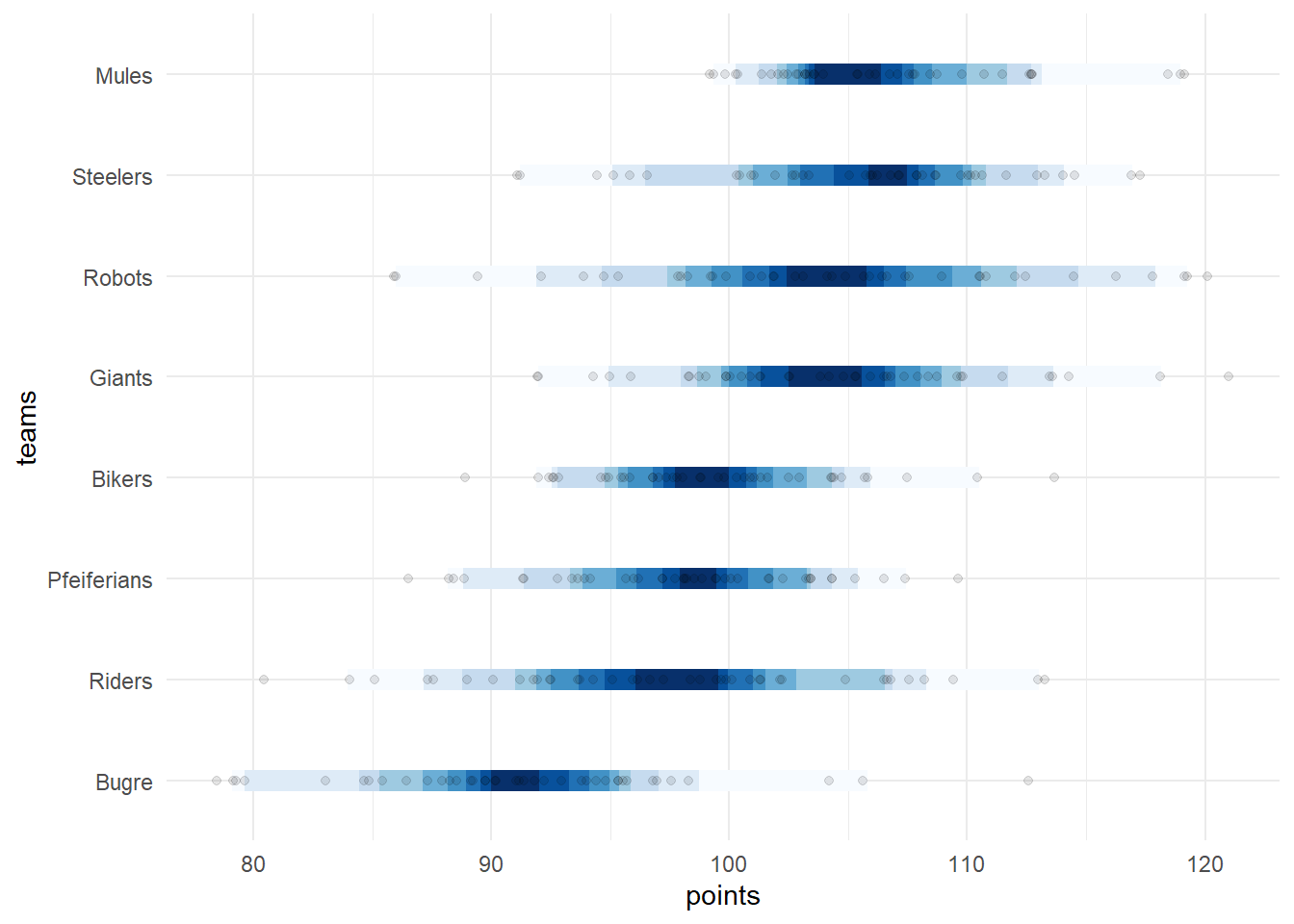

Showing the distribution of points instead of just the most probable score it is possible to see more details about the possibles performances of a team. The same can be visualized with the chances of victory, instead of just counting the number of times that the simulations of the matches point to the victory of a team, we can visualize the distribution of the difference in the score in each game, generating a curve of probability for each possible outcome.

simulation %>% 
  mutate(game=paste0(away.nickname, " @ ", home.nickname)) %>% 
  arrange(away.nickname) %>% 
  select(game, score.diff) %>%
  unnest() %>% 
  ggplot(aes(fill=game)) +
  geom_density(aes(score.diff), alpha=.6) +
  geom_vline(aes(xintercept=0),
             linetype=2, color="red") +
  facet_grid(rows=vars(game), switch = "x") +
  theme_minimal() +
  theme( legend.position = "bottom" )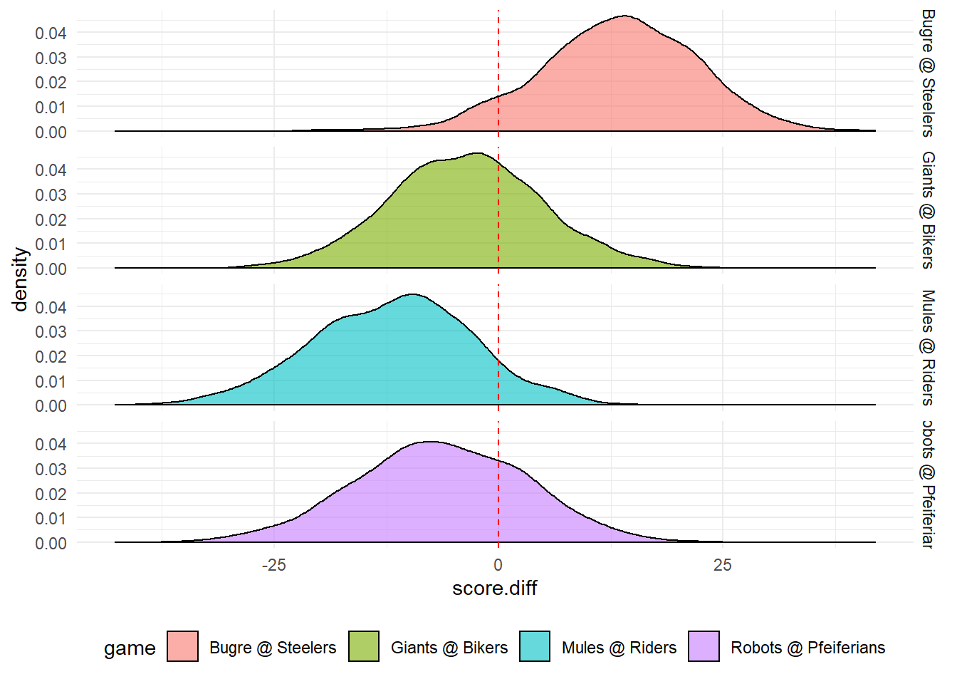

simulation %>% 
  arrange(away.nickname) %>% 
  mutate_at(vars(away.win.prob, home.win.prob), function(x) round(100*x,1)) %>% 
  select(away.nickname, away.win.prob, home.win.prob, home.nickname)  %>% 
   kable() %>%
   kable_styling(bootstrap_options = "striped", full_width = F)

away.nickname	away.win.prob	home.win.prob	home.nickname
Bugre	7.4	92.5	Steelers
Giants	67.2	32.8	Bikers
Mules	91.8	8.2	Riders
Robots	74.4	25.6	Pfeiferians

Conclusion

We have seen that it is possible to use NFL players’ performance projections, available on various websites, to calculate fantasy scores and to simulate, using Monte Carlo, the outcame of a league games. More sophisticated simulation models can be used, taking into account the historical distribution of the accuracy of the estimates of these sites to calculate a greater number of results possibilities.

Today, in my league, before the start of the round, after waivers and the lineups, I I send a dashboard (made using RMarkdown and Flexdashboard) to members with simulation results and the performance of their rosters. You can see an example of it here: http://rpubs.com/gsposito/ffsimulationDudes]. As an evolution, in the future, I may tranform this in to a ShinyApp to members be abble to simulate several different rosters combinations to choose the most promising one.

Prediction Evaluation

Before concluding it is worth comparing the simulation made with the actual scores, and evaluating how much the simulation projected came close to the obtained real result.

# comparing simulated values with real values
simulation %>% 
  mutate( 
    away.win.real   = away.pts > home.pts,
    home.win.real   = home.pts > away.pts,
    score.diff.real = home.pts - away.pts,
    away.sim.pts = map_dbl(away.sim.pts, median, na.rm=T),
    home.sim.pts = map_dbl(home.sim.pts, median, na.rm=T),
    score.diff   = map_dbl(score.diff, median, na.rm=T )
  ) %>% 
  mutate_at( vars(away.win.prob, home.win.prob), function(x) round(100*x,2) )%>% 
  select( away.nickname, away.win.prob, away.win.real, away.sim.pts, away.pts, score.diff, score.diff.real, 
          home.pts, home.sim.pts, home.win.real, home.win.prob, home.nickname ) %>% 
  mutate_if(is.numeric, round, digits=1) %>% 
  arrange(away.nickname) %>% 
   kable() %>%
   kable_styling(bootstrap_options = "striped", full_width = F)

away.nickname	away.win.prob	away.win.real	away.sim.pts	away.pts	score.diff	score.diff.real	home.pts	home.sim.pts	home.win.real	home.win.prob	home.nickname
Bugre	7.5	FALSE	92.3	112.6	13.6	13.7	126.3	106.3	TRUE	92.5	Steelers
Giants	67.2	TRUE	103.9	108.7	-3.6	-11.5	97.2	100.0	FALSE	32.8	Bikers
Mules	91.8	TRUE	106.7	98.4	-11.4	-8.3	90.1	95.3	FALSE	8.2	Riders
Robots	74.4	TRUE	104.9	113.6	-6.4	-30.4	83.1	98.1	FALSE	25.6	Pfeiferians

This was good! The simulated results were satisfactorily close to those obtained in 3 of the 4 games. All victories and defeats were correctly predicted. Only one of the games got a score difference far away from the one projected.

# comparing score difference
simulation %>% 
  mutate(
    game=paste0(away.nickname, " @ ", home.nickname),
    score.diff.real = home.pts - away.pts
  ) %>% 
  arrange(away.nickname) %>% 
  select(game, score.diff, score.diff.real) %>%
  unnest() %>% 
  ggplot(aes(fill=game)) +
  geom_density(aes(score.diff), alpha=.6) +
  geom_vline(aes(xintercept=score.diff.real),
             linetype=1, size=1, color="black") +
  geom_vline(aes(xintercept=0),
             linetype=2, color="red") +
  facet_grid(rows=vars(game), switch = "x") +
  theme_minimal() +
  theme( legend.position = "bottom" )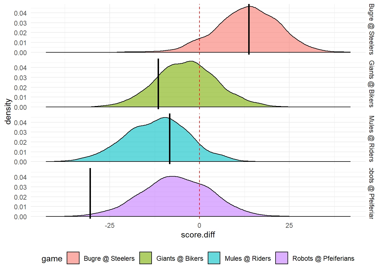

Perhaps the reason why the difference in scoring in the game between Robots and Pfeiferians has fallen so far from the most likely is also by such an unlikely event in the Packers’ game against the Lions. Here’s the lineup of the house team, the one who lost:

# rosted home team
simulation[1,]$home.roster[[1]] %>% 
  filter(rosterSlot != "BN") %>% 
  mutate(points.sim = map_dbl(sim.player,median, na.rm=T)) %>% 
  select(name, position, points) %>% 
   kable() %>%
   kable_styling(bootstrap_options = "striped", full_width = F)

name	position	points
Patrick Mahomes	QB	15.82
Adrian Peterson	RB	4.20
James White	RB	13.70
Antonio Brown	WR	22.10
Michael Thomas	WR	7.40
George Kittle	TE	8.30
Alex Collins	RB	6.60
Mason Crosby	K	3.00
Green Bay Packers	DEF	2.00

In this game, Mason Crosby, Packers’ Kicker missed 4 fields goals and 1 extra point, with a total of 13 points, an event rare, which has not happened since 1997. If Crosby had hit the shots, which he habitually does, the score difference would be only 10 points away from the predicted score, not 23!

But after all, who wants to predict accurately all possible situations?